Linear Regression Assumptions: What You Need to Know
Four essential checks, what each protects, and what to do if one fails


The 30-second summary
Linear regression rests on four assumptions about its errors, which you check mainly through your residuals, the gaps between what your model predicts and what you observed. You check three with plots and one with your study design.
- Linearity. The relationship is a straight line. A curve in the residual plot says it isn't.
- Independence. Each observation's error is unrelated to the others. Your study design settles this.
- Normality. The residuals, not your variables, are roughly normal. It matters most in small samples.
- Equal variance. The residuals spread evenly. A funnel means heteroscedasticity; robust standard errors handle it.
New to statistics? Our free statistics cheat sheet explains the main tests in plain English, on one page.
Navigate
Your advisor (your supervisor, in the UK) reads your results chapter and writes one line in the margin: check your assumptions. You run the regression again, find a residual plot in the output, and stare at a cloud of dots with no idea what it’s meant to show. You’re in good company: in a review of 172 clinical psychology papers that used regression, only 2% were both transparent and correct about their assumptions, according to Ernst and Albers (2017).
Having helped 10,000+ students through their dissertations, we’ve found that this is one of the most common points where a quantitative chapter stalls. In this post, I’ll explain the four assumptions of linear regression, show you what each check looks like when it passes and when it fails, and work through one dataset from start to finish, including how to fix the most common problem, heteroscedasticity.
The four assumptions of linear regression
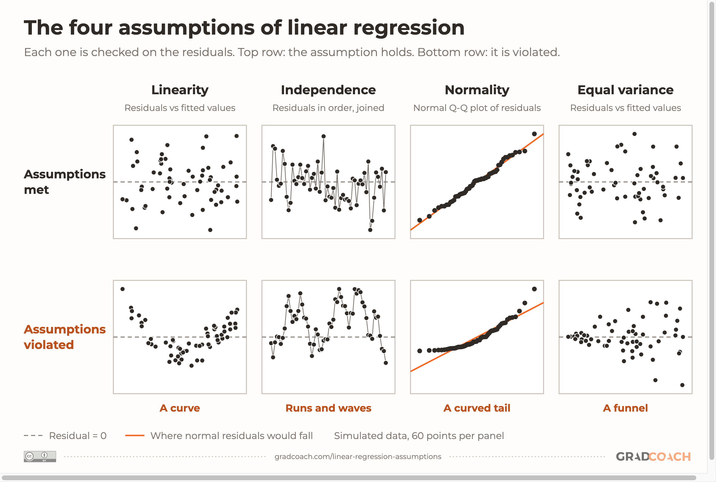
Strictly speaking, linear regression makes four assumptions about the model’s errors: the gaps between the true relationship and each observation. You can’t see the errors, so you check them using the residuals: the gaps between the values your model predicts (its fitted values) and the values you actually observed. Students often remember the four as LINE, the mnemonic used in Introduction to Modern Statistics:
- Linearity: The relationship between your predictor and your outcome is a straight line (or, in multiple regression, a straight-line combination of the predictors).
- Independence: Each observation’s error is unrelated to every other observation’s error.
- Normality: The errors are roughly normally distributed.
- Equal variance: The errors spread out by about the same amount at every level of the predictor. This is also called homoscedasticity.
The figure below shows each one twice: once when it holds and once when it’s violated.

Notice what isn’t on the list. Your variables don’t need to be normally distributed, only the errors do (which you check using the residuals). Williams and colleagues (2013) made this one of the two misconceptions their paper set out to correct, and the habit persists: in a 2025 review of 95 health research papers by Jones and colleagues, only 5 of the 28 that checked normality did so on the residuals. Most of the rest tested the variables themselves, or didn’t say what they tested.
What a violation actually breaks
Not every violation does the same damage. Some problems bias the coefficients themselves, so the slope you report is wrong. Others leave the slope unbiased (right on average) but make your standard errors (the model’s estimate of how precise each coefficient is), p-values and confidence intervals unreliable.
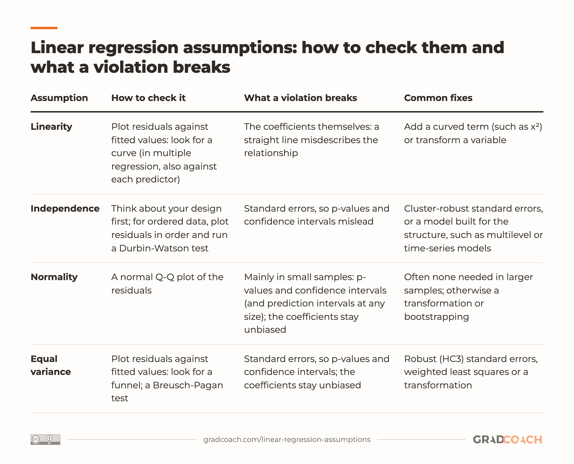
Knowing which is which tells you how worried to be and what to do. The table below sets out, for each assumption, how to check it, what a violation breaks and the usual fixes. Don’t worry if some of the test names are new; the worked example walks through each one:
| Assumption | How to check it | What a violation breaks | Common fixes |
|---|---|---|---|
| Linearity | Plot residuals against fitted values: look for a curve (in multiple regression, also against each predictor) | The coefficients themselves: a straight line misdescribes the relationship | Add a curved term (such as x²) or transform a variable |
| Independence | Think about your design first; for ordered data, plot residuals in order and run a Durbin-Watson test | Standard errors, so p-values and confidence intervals mislead | Cluster-robust standard errors, or a model built for the structure, such as multilevel or time-series models |
| Normality | A normal Q-Q plot of the residuals | Mainly in small samples: p-values and confidence intervals (and prediction intervals at any size); the coefficients stay unbiased | Often none needed in larger samples; otherwise a transformation or bootstrapping |
| Equal variance | Plot residuals against fitted values: look for a funnel; a Breusch-Pagan test | Standard errors, so p-values and confidence intervals; the coefficients stay unbiased | Robust (HC3) standard errors, weighted least squares or a transformation |
Two rows in that table deserve a closer look.
Independence is mostly a design question. If you surveyed 200 unrelated people once each, your observations are probably independent, and no plot will tell you much more.
The trouble starts when observations come in clusters (students in the same classes, patients in the same clinics) or in a sequence over time. Introduction to Modern Statistics calls independence often the most crucial assumption, and also the most difficult to diagnose. That’s why you settle it when you design your study, not when you analyze it. The Durbin-Watson test, which checks whether each residual is related to the one before it, only makes sense when your rows have a natural order, such as time.
Normality matters less than many students expect. Normal errors aren’t needed for your coefficients to be unbiased. They matter for the p-values and confidence intervals, and mainly in small samples: as Williams and colleagues put it, “the larger the sample, the lesser the importance of this assumption.” The Jones study goes further, calling normality the least important of the four.
A worked example: income and spending
I’ll run all four checks on one dataset. Suppose you’re studying how household income relates to monthly spending, and you’ve collected data from 150 households: annual income, in thousands of dollars, and monthly spending, in dollars. The data are simulated, so you can see each pattern clearly, but the shape is a familiar one: higher-income households spend more on average, and they also vary more in how much they spend.
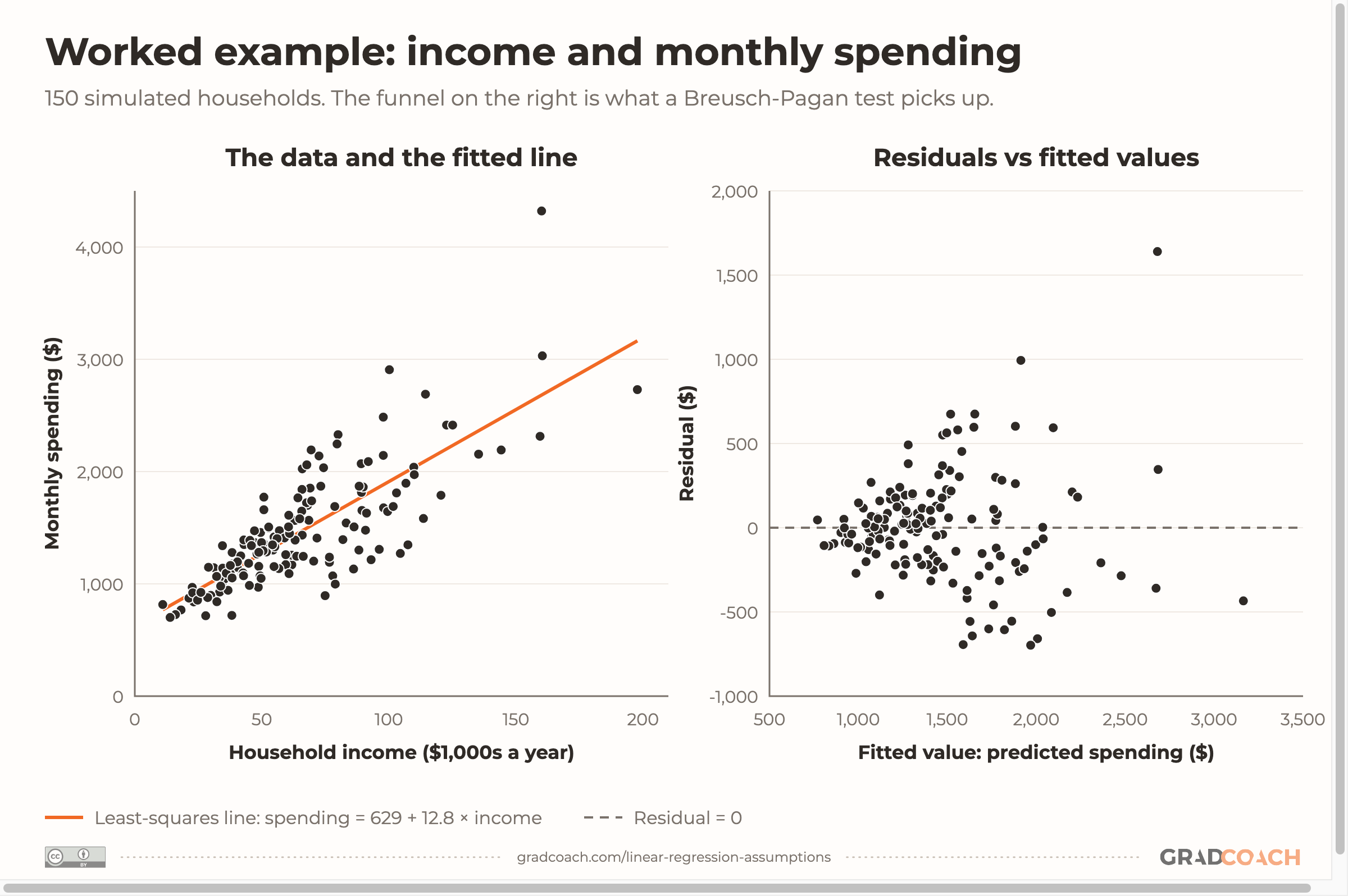
The regression gives a slope of 12.82: each extra $1,000 of annual income goes with about $12.82 more spending a month. The model explains 63% of the variance in spending (R² = .63). The figure below shows the data (left) and its residual plot (right): each household’s residual plotted against its fitted value. Watch how the spread widens as income rises:

If you use SPSS, you’ll find the main tools in Analyze > Regression > Linear. Under Plots, put *ZRESID (the standardized residuals) on the Y axis and *ZPRED (the standardized predicted values) on the X axis: that’s the residual plot. The Normal probability plot option in the same dialog is a P-P plot, not the Q-Q plot this post uses. For a Q-Q plot, tick Standardized residuals under Save, then run Analyze > Descriptive Statistics > Q-Q Plots on the new variable. Now take the four checks in turn.
1. Linearity
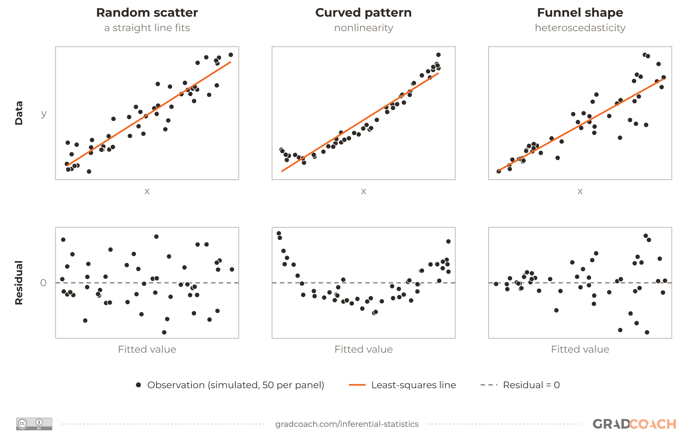
Look at the residual plot for a curve: residuals above zero at both ends and below it in the middle (or the reverse). There isn’t one here. The residuals center on zero all the way along, so a straight line is a reasonable description of the relationship. If you’re unsure what to look for, these residual plot examples show a good fit, a curve and a funnel side by side:

2. Independence
Our 150 households were each measured once, and none is linked to another (no shared addresses, no repeated measurements). So independence holds by design. The Durbin-Watson statistic is 1.94, close to the 2 you’d expect when neighboring residuals are unrelated, but with no natural order to the rows, it isn’t telling you much.
3. Normality
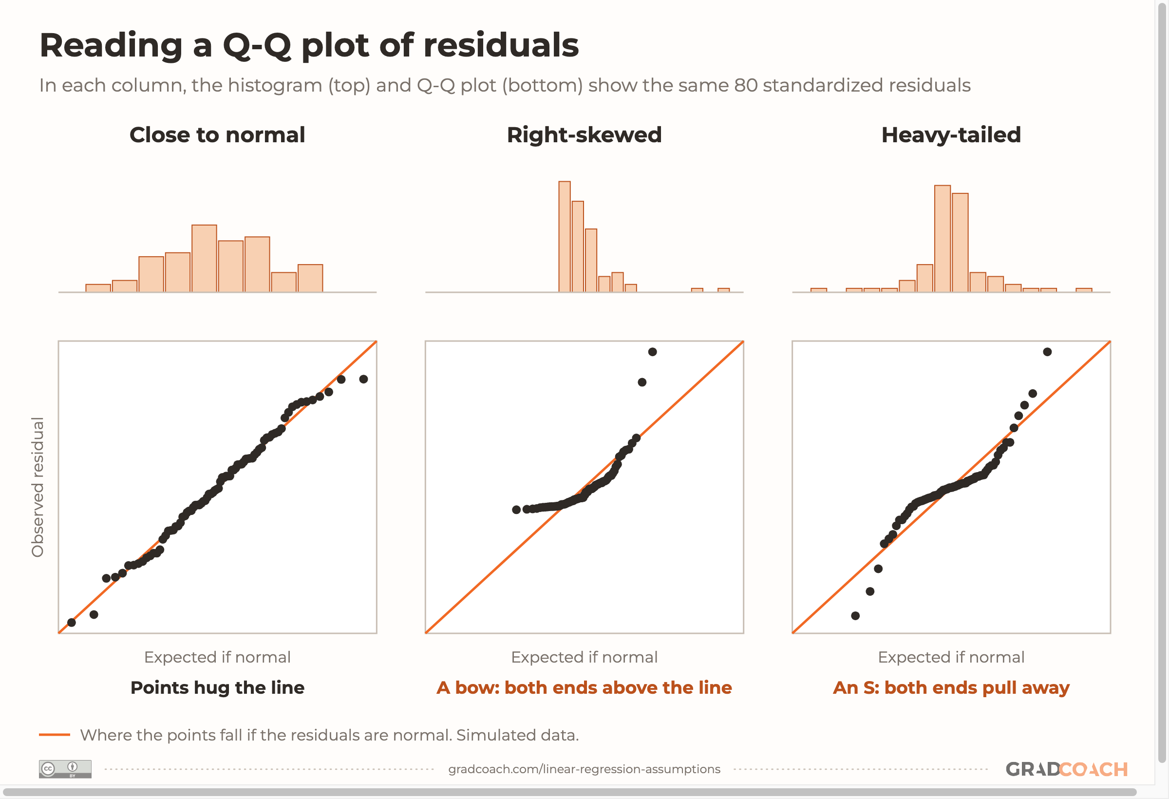
A normal Q-Q plot puts your residuals, sorted from smallest to largest, against the values a normal distribution would give. If the residuals are normal, the points fall along a straight reference line. The shape of any departure tells you what kind of problem you have:

In our example, the residuals’ Q-Q plot (not shown) bends away from the line, and a Shapiro-Wilk test, a formal test of normality, agrees (W = .94, p < .001).
Most of that is the funnel showing up again. The two largest residuals, both at high incomes where the spread is widest, give the residuals a long right tail; set them aside and the rest look close to normal. When some residuals come from a much wider spread than others, pooling them all tends to produce heavier tails than a normal distribution would.
It isn’t a serious problem here. With 150 observations, the p-values are fairly robust to it, and the fix for the funnel, robust standard errors (explained below), doesn’t rely on normal errors either in a sample this size.
In general, trust the Q-Q plot over a formal test. As Barker and Shaw (2015) point out, formal tests can flag trivial departures in large samples and miss real ones in small samples, and Jones and colleagues recommend judging residuals with a Q-Q plot rather than a statistical test.
4. Equal variance
This is where the model fails. The residual plot opens into a clear funnel, and the numbers confirm it: split the fitted values into thirds, and the residuals’ standard deviation grows from about $136 to $234 to $478. A Breusch-Pagan test, which checks whether the size of the residuals changes with the predictor, agrees (χ² = 25.4, p < .001). This is heteroscedasticity, which I’ll explain in full below.
That χ² of 25.4 comes from Koenker’s studentized version of the test, the default in R. The original version gives a larger statistic on the same data, so say which one you used.
One more check is worth making before you move on: unusual cases. A single household far from the rest can pull the slope on its own. Most statistics packages, SPSS included, can report Cook’s distance for each case, a measure of how much the fitted model changes when that case is left out. Investigate any case that stands well above the others before you think about removing it.
In this example, one household stands out: an income of $160,100 with spending of $4,321 a month (Cook’s distance 0.99; no other case is above 0.15). Nothing suggests it’s an error, and high spenders at high incomes are exactly what the funnel predicts, so it stays in. Without it, the slope falls from 12.82 to 11.73, still inside the robust confidence interval you’ll see below.
Homoscedasticity vs heteroscedasticity
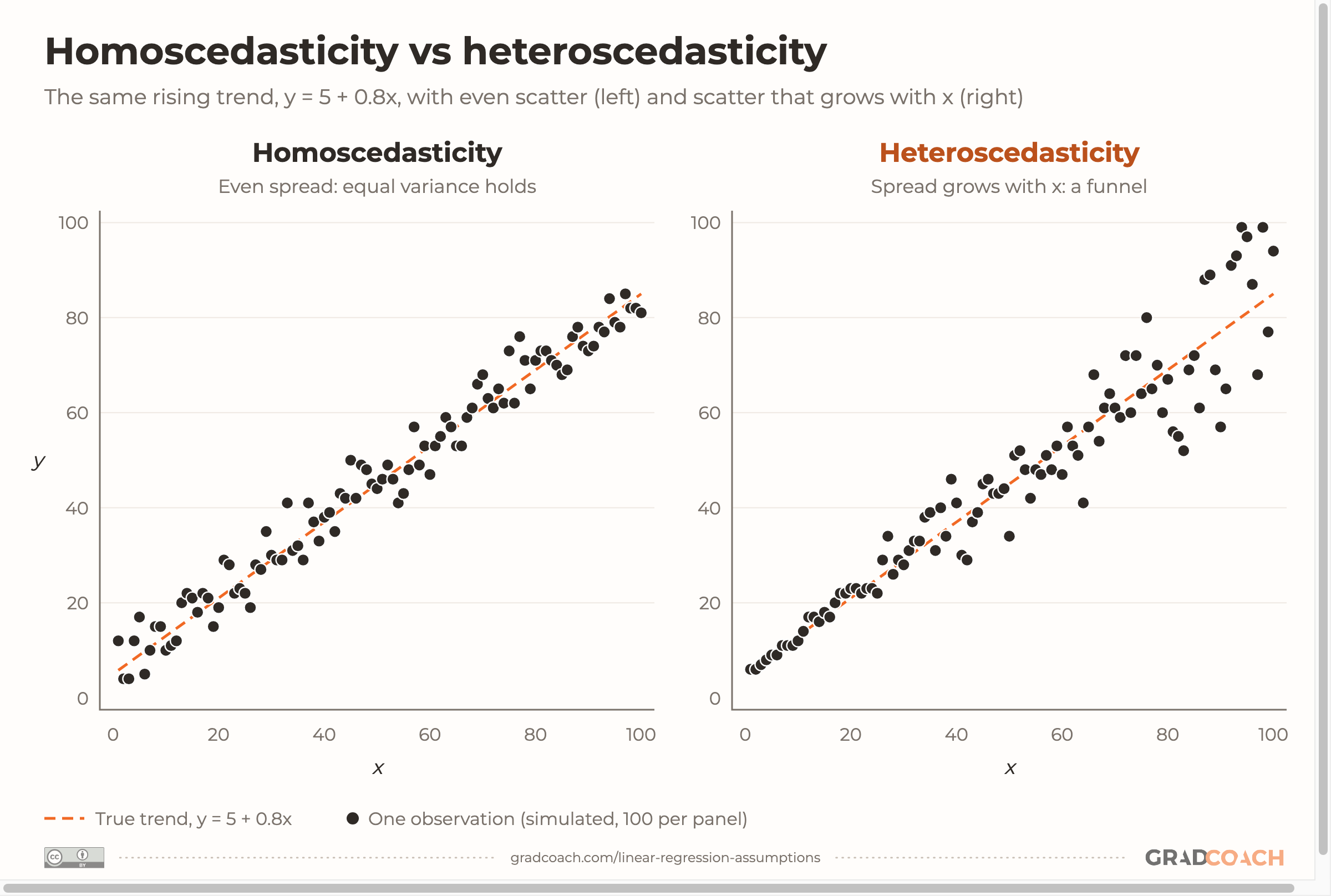
Homoscedasticity means the errors have the same spread, or variance, at every level of your predictor (which you check using the residuals). Heteroscedasticity means they don’t: the spread changes, usually growing as the predicted value grows. The figure below shows the same rising trend both ways:

So what does heteroscedasticity break? A common misunderstanding is that it biases your coefficients. It doesn’t: your slope is still right on average, as long as the rest of the model is right. What goes wrong is your measure of how precise that slope is. As Williams and colleagues explain, the usual confidence intervals and t-tests “can no longer be justified” when the errors don’t have equal variance. Your standard errors could be too small or too large, and your p-values and confidence intervals inherit the error.
Heteroscedasticity is common in data where the outcome grows with the predictor: spending and income, firm size and revenue, or counts that grow with time or population size. The bigger the values, the more room there is to vary.
One warning about the Breusch-Pagan test. Like normality tests, it’s sensitive to sample size: Jones and colleagues note that it’s prone to over-detecting minor deviations in large samples, and may lack power in small ones. So trust the plot first, and use the test as supporting evidence, not as the decision.
How to fix heteroscedasticity
You have three main options, and for most dissertations the first is the simplest.
1. Robust standard errors. Keep your regression exactly as it is, and replace the usual standard errors with heteroscedasticity-consistent ones, which don’t assume equal variance. A version called HC3 is a common choice: Long and Ervin found it worked well even with 25 observations, and advised using robust standard errors whenever you have reason to suspect heteroscedasticity, rather than waiting for a test to confirm it.
2. Weighted least squares. Give observations with more variable outcomes less weight in the fit. If you model the variance correctly, this gives more precise estimates than ordinary regression with robust standard errors. But you need to specify how the variance changes, which adds a decision you’ll have to defend.
3. A transformation. Taking the log of your outcome often evens out the spread, but it changes what your coefficient means: you’re now modeling proportional changes, not dollar changes. Make sure that still answers your research question.
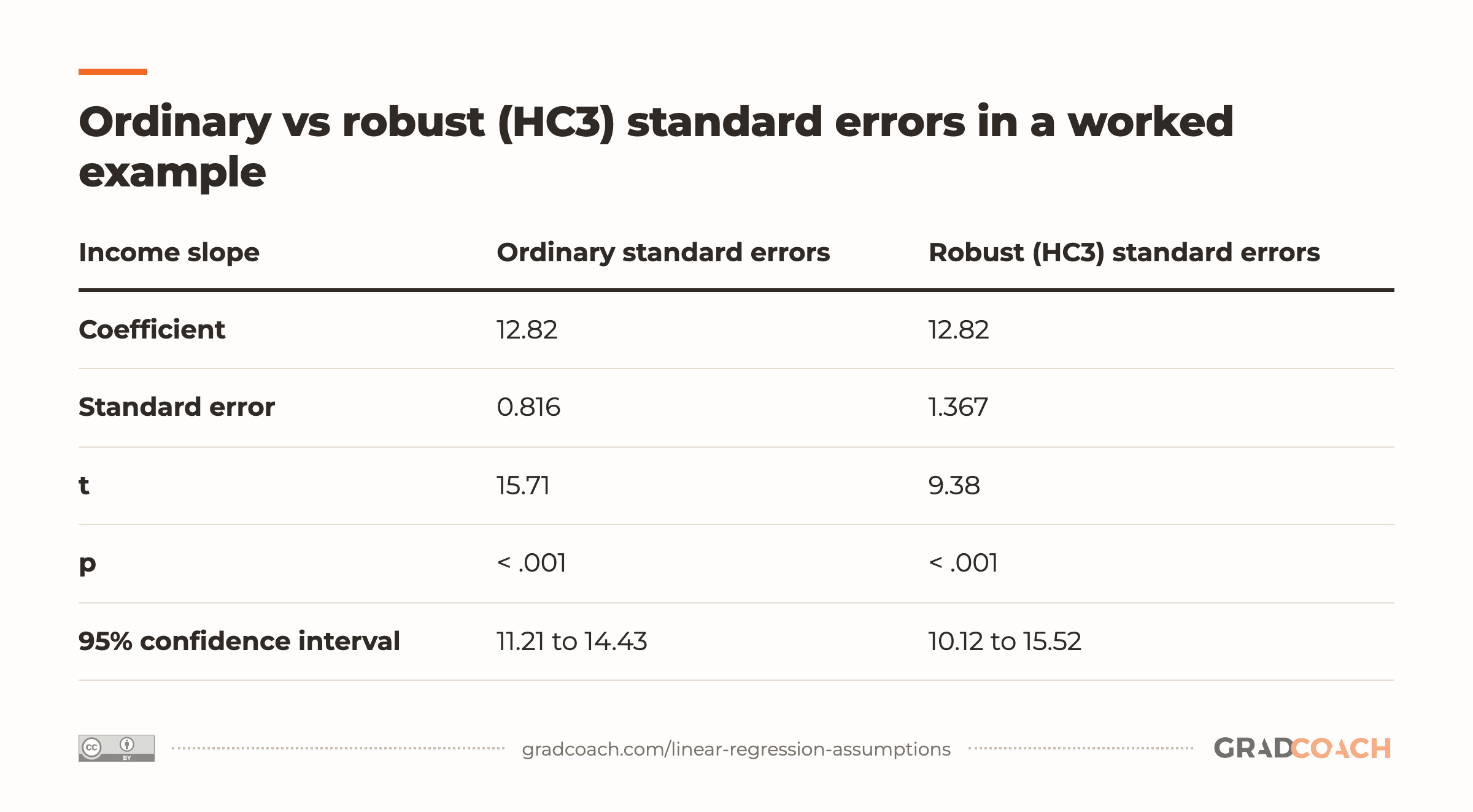
Here’s what robust standard errors do to the example. The slope doesn’t change at all, but its standard error grows by about two-thirds, and so does the width of its confidence interval:
| Income slope | Ordinary standard errors | Robust (HC3) standard errors |
|---|---|---|
| Coefficient | 12.82 | 12.82 |
| Standard error | 0.816 | 1.367 |
| t | 15.71 | 9.38 |
| p | < .001 | < .001 |
| 95% confidence interval | 11.21 to 14.43 | 10.12 to 15.52 |
In this example, the slope is still clearly significant either way. But the ordinary standard errors claimed much more precision than the data support: a reader would see a 95% confidence interval for the slope of $11.21 to $14.43 per $1,000 of income, when the robust interval runs from $10.12 to $15.52. With a weaker relationship or a smaller sample, the same correction could move a result across the .05 significance threshold, which is exactly why you check.
In SPSS (version 25 and later), you can get robust standard errors through Analyze > General Linear Model > Univariate. Put your outcome in Dependent Variable and your predictor in Covariate(s), then under Options tick Parameter estimates with robust standard errors and choose HC3. With continuous predictors entered as covariates, this gives the same coefficients as the Linear Regression procedure. The same dialog also offers tests for heteroscedasticity (SPSS spells it with a k).
In R, the sandwich and lmtest packages do the same job; in Stata, add vce(hc3) to your regression command.
What about multicollinearity?
Many lists of regression assumptions add a fifth: no multicollinearity, meaning two or more of your predictors are so closely related that the model can’t separate their effects. It’s worth checking in multiple regression, but it isn’t an assumption about the errors. It doesn’t apply to simple regression at all, because a model with one predictor has nothing to overlap with. Williams and colleagues suggest it’s “perhaps not best described” as an assumption.
Your overall model may still predict well, but the individual coefficients become unstable and their standard errors grow much larger. The usual check is the variance inflation factor (VIF), which measures how much that overlap inflates the variance of each coefficient (its standard error grows by the square root of the VIF). In SPSS, tick Collinearity diagnostics under Statistics in the Linear Regression dialog. You’ll see cutoffs of 5 or 10 quoted as “too high”, but treat those as conventions, not rules.
One mistake our coaches often see: treating any significant correlation between two predictors as a multicollinearity problem. Predictors are allowed to correlate. It’s only very high overlap that causes trouble, and the VIF is a better guide to that than a significance test on the correlation.
How to report your assumption checks
Assumption checks often fall down in the write-up, not because the checks were wrong, but because they’re invisible: no plot, no statement, or a single line saying “all assumptions were met.” In Jones and colleagues’ 2025 review of health research papers, 63% reported no assumption checks at all. It’s common to treat the checks as a pass-or-fail hurdle to clear and forget, when the examiner wants to see what you looked at and what you decided. A short paragraph covers it. For the income example, it might read:
Assumptions were checked using residual plots. The residuals showed no curvature, indicating a linear relationship, and observations were independent by design. Residuals were right-skewed and their variance increased with predicted spending (Koenker’s studentized Breusch-Pagan χ²(1) = 25.4, p < .001). Given the sample size (n = 150), the skew was not expected to affect inference materially. One influential case (Cook’s D = 0.99) was retained; excluding it reduced the slope from 12.82 to 11.73 without changing the conclusions. Because heteroscedasticity can make the usual standard errors unreliable, inference is based on HC3 heteroscedasticity-consistent standard errors.
Then report your coefficients with the robust standard errors, and put the residual plot in your chapter or an appendix. This paragraph belongs in your results chapter, next to the model it describes. If a decision could have gone either way, such as keeping an outlier, a useful approach is to run the model both ways and report that the results don’t differ (or explain how they do). Whether an outlier should be removed at all is a judgment call of its own.
The checks themselves take minutes. What takes practice is reading the plots and deciding what to do about what you see. If you’d like a second pair of eyes on your model, our coaches help students with dissertation statistics, whether that’s reading the plots or defending a choice to your examiner.
Still have questions?
What are the four assumptions of linear regression?
Linearity, independence, normality and equal variance, often remembered as LINE. Strictly speaking, all four are about the model’s errors, and you check them using the residuals: the differences between the observed values and the values the model predicts. Some lists add “no multicollinearity” as a fifth, but that’s a property of the predictors in multiple regression, not an assumption about the errors.
Do my variables need to be normally distributed?
No. Linear regression assumes the errors are roughly normal, which you check on the residuals, not the predictor or outcome variables. A skewed predictor is fine. Even residual normality matters mainly for p-values and confidence intervals in small samples, and it doesn’t affect whether the coefficients are unbiased.
Is heteroscedasticity good or bad?
It’s a problem for inference, not for the coefficients. Heteroscedasticity leaves the regression coefficients unbiased, but it makes the usual standard errors, p-values and confidence intervals unreliable. Homoscedasticity, equal variance in the residuals, is what ordinary least squares assumes. Robust (HC3) standard errors are the simplest fix when it fails.
How do I check homoscedasticity in SPSS?
Ask for a plot of the standardized residuals (*ZRESID) against the standardized predicted values (*ZPRED) under Plots in the linear regression dialog, and look for a funnel shape. In SPSS 25 and later, the General Linear Model Univariate procedure also offers heteroskedasticity tests and robust standard errors under Options.
What if my residuals aren’t normal?
First check the other assumptions, because a funnel or a curve can make the residuals look non-normal. In a larger sample, mild non-normality rarely matters for your p-values. In a small one, consider a transformation or bootstrapped confidence intervals, and say in your write-up what you saw and why you chose what you did.
Is multicollinearity an assumption of linear regression?
Not strictly. It’s a property of the predictors, and it only applies to multiple regression. Very high overlap between predictors makes individual coefficients unstable, so it’s worth checking with the variance inflation factor (VIF), but a significant correlation between two predictors isn’t a problem in itself.
What is the Breusch-Pagan test?
A test for heteroscedasticity. It checks whether the squared residuals of a regression are related to the predictors, which would mean the error variance changes. A significant result suggests heteroscedasticity, but in large samples it can flag differences too small to matter, so read it alongside a residual plot.
Can’t find your answer here? Ask a Grad Coach directly – the initial chat is free.
Speak with a friendly coach →


Cite-worthy sources
Cite this article
Jansen, D. (2026). Linear Regression Assumptions: What You Need to Know. Grad Coach. https://gradcoach.com/linear-regression-assumptions/
- Barker, L. E., & Shaw, K. M. (2015). Best (but oft-forgotten) practices: Checking assumptions concerning regression residuals. The American Journal of Clinical Nutrition, 102(3), 533-539.
- Çetinkaya-Rundel, M., & Hardin, J. (2024). Introduction to modern statistics (2nd ed.). OpenIntro.
- Ernst, A. F., & Albers, C. J. (2017). Regression assumptions in clinical psychology research practice: A systematic review of common misconceptions. PeerJ, 5, e3323.
- Jones, L., Barnett, A., & Vagenas, D. (2025). Common misconceptions held by health researchers when interpreting linear regression assumptions, a cross-sectional study. PLOS ONE, 20(6), e0299617.
- Long, J. S., & Ervin, L. H. (2000). Using heteroscedasticity consistent standard errors in the linear regression model. The American Statistician, 54(3), 217-224.
- Williams, M. N., Gómez Grajales, C. A., & Kurkiewicz, D. (2013). Assumptions of multiple regression: Correcting two misconceptions. Practical Assessment, Research & Evaluation, 18(11).